In the book The Phoenix Project there is a part where Bill is discussing lead times with Wes and Patty. Even though a certain task only takes 30 seconds, the lead time is still hours due to the time spent waiting for a resource to become available (Brent). Bill draws a graph to demonstrate the problem: if a resource is fully (100%) utilised then wait times become very long.

This statement threw me for a bit until I did some research. The graph definitely nails the problem with trying to maximise utilisation of resources. I mean, it is counter-intuitive for a manager to allow resources to idle. So what is the graph actually showing?
The graph shows that when the average utilisation goes over 80-90% then wait times become very long. So over time, a very high average utilisation will cause the queue to grow very long, increasing lead times dramatically. In other words, if a resource is very busy then it cannot cope with a workload that varies. The team must be allowed some slack so that lead times are still reasonable even when the workload is sometimes higher than average. In short, there is a trade-off between workload variability and resource utilisation.
This is well-understood in the manufacturing industry, but it is intrinsically true for software development. Everything that is built in software development is a one-off, unique. This creates huge variability in the job times of the development process; no two projects are ever the same. The challenge then is to reduce this variability so that we can create a more predictable workload and push up utilisation.
In Agile we use techniques such as storyboarding, MVPs and backlog grooming to manage variability and ensure that we maintain flow. WIP limits and Velocity are our KPIs that let us know how well we are succeeding in maintaining flow. Flow refers both to managing the variability of the arrival time of work (i.e. breaking down the work into smaller deliverables) and the execution time of the job (e.g. sizing of User Stories).
The science
Back to Bill’s graph. Where does it come from? It is actually based on Kingsman’s formula which is from the domain of queueing theory. In layman’s terms the wait time is made up of three parts:

So what Bill is actually saying is that, given a certain variability and a certain job time, then the wait time will be a function of the utilisation as shown in the graph above. Bill wants to focus on utilisation, so he normalises the other parameters (variation and job time) as follows:

For an excellent explanation of the Kingsman’s formula have a look at EuroLEAN+’s Youtube tutorials.
Reducing variability
Variation is the norm in software development, so it has to be dealt with. There are several ways to mitigate variability. Reducing utilisation is one option, but we can do better than having our developers and testers idling.
Kingsman’s formula shows that adding more work centres reduces sensitivity to variation (as well as increasing capacity obviously). However, this is probably more feasible in manufacturing than in software development, because a work centre (i.e. a development team) often has domain expertise, i.e. no two teams have exactly the same capabilities. But this approach may be more applicable in larger organisations.
We have already mentioned reducing variability using Agile techniques such as storyboarding, MVPs and backlog grooming, and this should be the primary focus of the team coach in creating and optimising flow.
Another option available to development teams is to have a technical backlog containing work that is lower priority that can be used to fill idle time and bring utilisation closer to 100%. The kind of tasks in this backlog should be small and independent. For example, it could involve refactoring, writing automated tests, learning about a new technology, and so on.
In summary, it is the combination of these techniques that allows development teams to be fully utilised. What Lean teaches us, is that the same discipline and structure that is used to optimise manufacturing flows, applies even more so to software development.
Tracking the team’s velocity gives us insights into both utilisation and the amount of planned work vs. unplanned work. We can also track the velocity of both Stories and Epics to see how good we are at sizing our MVPs. (An Epic is always an MVP in my book; this makes it clear what the definition of Done is for an Epic).
Skipping the queue
One of the early problems Bill had to deal with was departments trying to skip the queue. This is the result of a chronic failure of the development process. If lead times become unacceptably long (due to high utilisation, high variability or both), then eventually people will try to find shortcuts. This just makes a bad problem even worse, and represents a total breakdown in the chain-of-command. That kind of short circuit has to dealt with before any other improvements have a chance of succeeding. Hence the need to start by visualising all of the work in process.
Inventory
I was almost going to write that inventory doesn’t cost anything in software development, after all it is virtual. We don’t have to purchase raw materials and we don’t have to store anything in warehouses. (Yes, GitHub costs something, but it is a negligible cost in this context.)
But there is still inventory in software. The raw materials are just ideas, one-liners that take up virtually no space at all and until the team commits to building (analysing, developing and testing) something, the backlog can be reorganised and priorities changed as often as desired.
The rest of the inventory is in the queues between work centres, e.g. when handing over from development to test. This inventory does represent an investment in time and effort, e.g. breaking down the problem, defining an MVP and coding a solution. The cost of having this inventory is that the knowledge about the solution disappears over time; no amount of documentation can replace the shared understanding that existed when the team were working actively on the solution. Furthermore, TTM is probably the single most important factor for success nowadays. So to sum up, a lot of inventory, or WIP, is bad in software development. Watch those WIP limits!
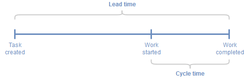
Cycle time
Here is an example of a good article describing Lead times and Cycle times. However, the difference between the two is not very clear in my opinion. A new Initiative will contain an unknown amount of work, that’s why we analyse it and break it down into reasonably sized chunks; we are reducing variability and minimising risk. A task (e.g. User story) is only added to the backlog when it is somewhat well-defined and so the Lead time for every deliverable is a reasonably well-understood and managed parameter. Otherwise, Lead times just becomes guess work and that is not so useful.
But the backlog doesn’t only contain planned work, it also contains unplanned work; bugs and outages which must be dealt with immediately. This increases the Lead time for planned work in ways that can be hard to manage. While unplanned work cannot be avoided completely, it can be mitigated using a small iterative release process, i.e. continuous delivery, continuous improvements to the delivery process, as well as detective and preventative security controls.
So ideally, Lead Time only applies to tasks that are MVP-sized and, we should also have a WIP limit on new work to control Lead time. It does not make sense to fill up the backlog with Tasks that will be delivered years from now. Doing this, we achieve an understanding of the team’s capacity and that long Lead times indicate the need for an increase in team capacity, the need for more teams, or a change in priorities.
My agile development team was involved in storyboarding and backlog grooming for all new tasks, not just development and testing. The team were constantly managing the flow of deliverables at all stages on the Kanban board, both when there were too few and too many tasks in a queue. So the difference between “Task created” and “Work started” was really very small, and therefore Cycle time should be uninteresting.
In queueing theory there is a formula known as Little’s Law which is used to calculate the Cycle time. So does this formula still have relevance even if we are not interested in Cycle time?

The term “Cycle time” is somewhat non-intuitive. But if you think about it, the cycle time is also the average time it will take to deliver everything that’s on your Kanban board right now. For example, if your WIP is 10 and your average throughput is 2 tasks/day, then your cycle time is 5 days/task. Or put another way, the team can deliver everything on the Kanban board within the next 5 days. Now that’s a rather powerful statement. So Cycle time is also the Turnover time for all WIP.

The better the team get at breaking down the backlog into equal-sized chunks (i.e. minimising variability), the more relevant the turnover figure becomes.
And so if Cycle times converge with Lead times, then we are much more sure of our commitments to the business side of the organisation. Roll-on Big Room Planning!